This is the multi-page printable view of this section. Click here to print.
Blog
- A Nobel Prize for Controlling the Brain with Light
- Suggesting Metadata Improvements to Dandiset Owners
- DANDI Notebooks: Persistent, Executable Companions to Neurophysiology Data
- Place Cells in Space: Hippocampal Recordings from the Space Shuttle
- Introducing DANDI Atlas Explorer: Explore the DANDI Archive in 3D
- NWB Compression Recommendations for DANDI Archive
- Unraveling Anesthesia's Effect on Brain Activity
- Human ex-vivo microscopy workshop/hackathon
- External Links in NWB and DANDI
- DANDI User Workshop
- DANDI: A data archive and collaboration space for neurophysiology
A Nobel Prize for Controlling the Brain with Light
How a protein from pond algae became one of the most important tools in brain science, and where you can see the data it produces.
On October 5, 2026, the Nobel Assembly at Karolinska Institutet awarded the Nobel Prize in Physiology or Medicine to Karl Deisseroth, Peter Hegemann and Georg Nagel. The citation is short: “for their discoveries concerning light-gated ion channels and optogenetics.”
Optogenetics lets scientists switch specific brain cells on or off with a flash of light. That sounds like science fiction. It is now an everyday method in thousands of laboratories, and it has changed what we can learn about memory, mood, movement and disease.
At the DANDI Archive, we see the results of this work every day. DANDI is a free public library of brain recordings, and many of the datasets shared here were made with the technology honored this week. This post explains what optogenetics is, where it came from, and how anyone can explore the experiments it made possible.
A light switch for brain cells
Your brain holds roughly 90 billion nerve cells, called neurons. They talk to each other with tiny electrical pulses. Every thought, memory and movement is a pattern of those pulses.
For most of the last century, scientists could watch this activity but could not control it precisely. They could see that a group of neurons was busy when an animal felt afraid. They could not prove those neurons caused the fear. Older tools, such as electrical stimulation or drugs, affected every cell in the neighborhood at once.
Optogenetics solves this with two ingredients, which give it its name:
- Genetics. Scientists give chosen neurons the instructions to build a light-sensitive protein. Only the cell type they pick receives it.
- Optics. A hair-thin optical fiber delivers light to that part of the brain. Neurons carrying the protein respond within thousandths of a second. Their neighbors do not.
Some of these proteins turn neurons on. Others turn them off. Researchers can now ask a direct question: what happens to behavior when this exact group of cells is switched on, or silenced, at this exact moment?
Think of the brain as a city at night. Earlier methods could show which neighborhoods were lit up. Optogenetics lets you flip the switch in a single house and see what changes.
It started with algae that swim toward light
The story does not begin in a brain lab. It begins with Chlamydomonas, a single-celled green alga found in ponds and soil. It has a tiny orange “eyespot” and swims toward light.
In the early 1990s, Peter Hegemann wondered how it reacts so quickly. He measured an electrical response half a millisecond after light hit the eyespot. That is more than twenty times faster than the human eye. He proposed that a single protein both catches light and lets electrical charge into the cell. Many colleagues were skeptical.
About a decade later, Hegemann teamed up with Georg Nagel. Nagel put two candidate algae genes into frog eggs and showed that Hegemann was right. They named the proteins channelrhodopsins, and described them in papers in 2002 and 2003. They also showed that other kinds of cells became light-sensitive when given the gene.
Karl Deisseroth, a psychiatrist and neuroscientist at Stanford, was looking for exactly such a protein. He wanted better ways to understand the illnesses he saw in his patients. He wrote to Nagel and asked for the DNA. In 2005, his group reported that rat neurons carrying the algae protein fired on command when lit with blue light. In 2007, they made it work in the brains of living mice, steering whisker movements through an optical fiber.
| Year | Milestone |
|---|---|
| Early 1990s | Hegemann measures the algae’s ultrafast response to light and proposes a light-gated channel |
| 2002–2003 | Nagel and Hegemann identify channelrhodopsin-1 and channelrhodopsin-2 |
| 2005 | Deisseroth’s group controls rat neurons in a dish with blue light |
| 2006 | The method gets its name: optogenetics |
| 2007 | First control of neurons in the brains of living mice |
| 2012 | Researchers reactivate a specific fear memory in mice |
| 2021 | A clinical trial reports partial recovery of vision in a blind patient with retinitis pigmentosa |
Dates are from the Nobel Committee’s popular science background.
Three names are on the prize, but many hands built the field. The 2005 paper was co-authored by Edward Boyden, Feng Zhang and Ernst Bamberg, alongside Nagel and Deisseroth. Hundreds of labs have since added new proteins, new colors of light and new ways to deliver them.
There is a lesson here about curiosity. Nobody studying pond algae in 1990 was trying to treat blindness or understand depression. Basic research paid off in a direction no one could have planned.
Optogenetics on the DANDI Archive
When a lab runs an optogenetics experiment, it records what the neurons and the animal did before, during and after each flash of light. Those recordings are the raw evidence behind the discoveries. More and more labs now share them openly on DANDI, so that anyone can check the results or ask new questions of the same data.
A search for “optogenetic” on DANDI returns 68 datasets as of October 5, 2026. Here are six that show the range of questions this tool can help answer.
| Question | What the researchers did | Dataset |
|---|---|---|
| How does the brain hold a plan in mind? | Mice had to wait a moment before licking left or right. Briefly silencing the motor cortex or the thalamus on one side with light biased their choices. Silencing either region also shut down activity in the other, suggesting the two keep the plan alive together. | DANDI:000009 (Svoboda lab, paper) |
| What does dopamine do when no reward is on offer? | Light was used to nudge dopamine at precise moments while mice roamed freely. Small boosts made the mice more likely to repeat whatever they had just been doing. | DANDI:000559 (Datta lab, paper) |
| How does a habit become a compulsion? | Turning dopamine signals up in one part of the striatum sped the shift to compulsive reward seeking in mice. Turning them down delayed it. | DANDI:000971 (Lerner lab, paper) |
| How do signals travel through a whole brain? | In a tiny worm, researchers lit up neurons one at a time and watched the rest of the brain respond. They measured 23,433 pairs of neurons and found signals that the wiring diagram alone did not predict. | DANDI:001075 (Leifer lab, paper) |
| How do neurons weigh their inputs? | Gentle light pulses were used to probe hippocampal neurons in freely moving mice, revealing hidden “place fields” in cells that had not shown one. | DANDI:000568 (Buzsáki lab, paper) |
| Could light calm overactive human brain tissue? | Slices of human hippocampus, donated by patients having epilepsy surgery, were given light-sensitive proteins. Light then lowered the tissue’s firing under conditions that provoke overactivity. | DANDI:001132 (paper) |
Several newer datasets apply the same tool to Parkinson’s disease. In DANDI:001933, light activates the dopamine neurons most vulnerable in the disease, to test how a Parkinson’s-linked gene affects them. DANDI:001832 uses light in brain slices to show how one circuit in the striatum is disrupted in parkinsonian mice. DANDI:001538 uses it to probe the involuntary movements that can follow long-term levodopa treatment.
Notice the pattern across these studies. Each one goes beyond watching the brain. It changes something specific and measures what follows. That move from correlation to cause is what the Nobel Committee recognized.
Why sharing the data matters
Optogenetics spread fast because its inventors shared it. Deisseroth got the channelrhodopsin DNA by writing to Nagel and asking. His lab then sent the tools to thousands of other labs.
Open data follows the same idea. Brain experiments are slow and costly, and most are paid for with public money. When the recordings are shared, other scientists can verify the findings, combine studies, and test ideas the original team never thought of. Students anywhere in the world can learn from real data.
DANDI is funded by the U.S. National Institutes of Health through the BRAIN Initiative. It holds more than 1,100 datasets and over 2 petabytes of data, free to anyone.
You do not need to be a scientist to look around:
- Browse the archive at dandiarchive.org and search for a topic such as “optogenetics,” “memory” or “Parkinson’s.”
- Open any dataset above to read its description and see who made it.
- If you write code, try the example notebooks that walk through loading and plotting real recordings.
Congratulations to Karl Deisseroth, Peter Hegemann and Georg Nagel, and to the many researchers whose work with their discovery fills this archive.
Sources and further reading
- Nobel Assembly at Karolinska Institutet: press release and popular science background, “A light-sensitive algal protein energised neuroscience”
- HHMI: Karl Deisseroth wins the 2026 Nobel Prize in Physiology or Medicine
- STAT: 2026 Nobel Prize in Medicine awarded for brain research tool called optogenetics
- Scientific American: 2026 Nobel Prize awarded for work on optogenetics
- Nagel et al., Channelrhodopsin-1: a light-gated proton channel in green algae, Science, 2002
- Nagel et al., Channelrhodopsin-2, a directly light-gated cation-selective membrane channel, PNAS, 2003
- Boyden et al., Millisecond-timescale, genetically targeted optical control of neural activity, Nature Neuroscience, 2005
- Sahel et al., Partial recovery of visual function in a blind patient after optogenetic therapy, Nature Medicine, 2021
- DANDI Archive: search results for “optogenetic”
Suggesting Metadata Improvements to Dandiset Owners
The metadata attached to a dandiset determines how well the data can be found, cited, and credited. When a dandiset lists the paper it supports, a reader who finds the paper can find the data and a reader who finds the data can find the paper. When contributors carry ORCID identifiers, the dataset shows up on their ORCID records. When funders are linked to their ROR records with award numbers, program officers can trace the data their grants produced. When the subject field names brain regions and conditions from standard ontologies, the dandiset can be found by searching for those terms.
Many dandisets are missing some of this. It is common to find a dandiset whose description cites a paper that is not listed as a related resource, whose authors have no ORCIDs, whose funders are listed only by name, and whose subject field is empty. Most of these fields are optional at upload time, the paper often comes out after the data is shared, and looking up a dozen ORCIDs and ontology terms by hand is tedious work that is easy to put off.
The DANDI Metadata Editor
We maintain a metadata editor at medit.dandiarchive.org. It loads the draft version of any dandiset, shows its metadata in an editable view, and includes a checklist that scores the metadata on the items above: license, authors, ORCIDs, affiliations, funders, subject terms, keywords, a linked publication, and ethics approval. It also has an AI assistant that can look up papers, ORCIDs, ROR records, and ontology terms and propose edits. Every edit is held as a pending change and shown as an inline diff, and nothing is written to the archive until an owner commits it with their own API key.
The editor can also package a set of pending changes as a proposal link. The link carries the changes and a hash of the metadata they were computed against, and opening it loads the dandiset with the changes applied and highlighted. Anyone can make a proposal link, but only an owner can commit it. If the dandiset has been edited since the link was made, the hash no longer matches and the editor refuses to apply the changes.
Proposing Changes Across the Archive
Proposal links make it possible to do the tedious part of the work for owners and leave them the decision. We have built a pipeline that does this across the archive. It runs the editor’s checklist on every open dandiset and ranks them by how much of what is missing could be filled in from public sources. For each dandiset near the top of that list, an AI assistant (Claude) reads the metadata and searches OpenAlex, Crossref, ROR, ORCID, the EBI Ontology Lookup Service, the Allen Mouse Brain Atlas, and the Cognitive Atlas for the missing information, then proposes a set of changes.
Those changes then pass through a set of checks written as ordinary code, separate from the AI. Every ORCID, ROR identifier, DOI, and ontology term in a proposal must have been returned by one of the lookups during that dandiset’s run, so an identifier the assistant invents or misremembers is rejected. A person can only be added as an author if they appear on a paper that is linked to the dandiset. Only structured fields may change: the title and description are never touched, existing contributors are never removed, and existing award numbers are left alone. A contact person is only proposed when the choice is unambiguous, for example when only one contributor has an email address; otherwise the email asks the owner to choose. The proposed metadata is validated against the DANDI schema and must not introduce any errors the draft did not already have. Proposals are capped at twelve changes so that the review stays short.
The pipeline builds the proposal link with the editor’s own hashing and diff code and drafts an email to the dandiset’s contact person. The email links to the dandiset, opens the editor with the proposed changes, lists each change in plain language, and explains the three steps to accept them: paste a DANDI API key into the editor, read through the highlighted changes and adjust or discard anything that looks wrong, and click commit. We read every draft before it is sent.
What It Found
The 88 proposals emailed so far suggest the following additions to the dandisets they cover:
| Change | Count |
|---|---|
| ORCIDs for existing contributors | 265 |
| Contributor affiliations linked to ROR | 187 |
| Funder entries with a ROR identifier | 171 |
| Subject terms from UBERON, the Cell Ontology, the Allen Mouse Brain Atlas, disease ontologies, and the Cognitive Atlas | 151 |
| Related publications and preprints | 86 |
| Authors added from a linked paper, with ORCIDs | 37 |
The most valuable single change is usually the paper. Once the assistant finds the publication a dandiset supports, OpenAlex returns the authors’ ORCIDs and institutions and the funders and award numbers acknowledged in the paper, so one lookup fills in most of the rest.
Owners Stay in Control
The emails started going out today, and a few owners have already committed some or all of the suggested changes. Because the proposal only applies to the exact version of the metadata it was built from, an owner can edit freely before or after, and a link that has gone stale simply stops working. An owner who disagrees with a change can discard it in the editor before committing, and we would like to hear about anything the assistant got wrong so that we can fix it in the pipeline as well as in the dandiset.
If you own a dandiset and have not received one of these emails, you can get the same help directly. Open your dandiset in medit.dandiarchive.org, look at the checklist, and ask the assistant to fill in what is missing.
DANDI Notebooks: Persistent, Executable Companions to Neurophysiology Data
A dataset on DANDI is most useful when it comes with code that shows how to read it and what can be done with it. For several years we have collected such notebooks at notebooks.dandiarchive.org: walkthroughs of individual dandisets, tutorials from workshops, and in a growing number of cases, notebooks that reproduce specific figures from the paper a dataset was published with.
The difficulty with notebooks has always been keeping them runnable. A notebook that worked when it was written depends on a particular set of package versions, and those versions drift. Within a year or two, a reader who tries to run it often finds that a dependency has changed its API, a default has moved, or a package no longer installs at all. The code is still there, but the ability to execute it has quietly evaporated.
We have now addressed this with two complementary ways to run every notebook in the collection, and the second of them changes what the collection can be used for.
Running a Notebook in Google Colab
Each notebook on the index carries an “Open in Colab” badge. Clicking it opens the notebook in Google Colab, where the first cell installs the notebook’s dependencies at fully pinned versions, not just the packages the notebook imports but their entire transitive closure, resolved against the versions Colab ships so that the install is fast and rarely requires a runtime restart. After that cell runs, every later cell executes against exactly the environment the notebook was tested in. Nothing needs to be installed on your own machine, and the data streams directly from the DANDI Archive.
This is the easiest path, and for a quick look at a dataset it is the one we expect most people to take. Its limitation is that it rests on an environment we do not control. Colab updates its Python version and preinstalled packages on its own schedule, and a pinned install that works today is not guaranteed to resolve on the Colab of a few years from now.
Running a Notebook in a Container
For that reason each notebook is also published as a container image. The image bundles the notebook, the exact pinned Python environment, a JupyterLab server, and any helper files, frozen together. Running one takes a single command:
docker run --rm -p 127.0.0.1:8888:8888 ghcr.io/dandi/example-notebooks/001550-paganlab:latest
JupyterLab opens in your browser on the notebook with everything already installed.
The images are built for both Intel and ARM processors, so they run natively on Apple
Silicon laptops as well as on Linux servers, and each image carries a date tag alongside
latest so that a specific snapshot can be cited in a methods section.
An image is only pushed to the registry after the notebook has been executed successfully inside it, on both processor architectures, as an unprivileged user, under a memory limit typical of a laptop. An image that is on the registry is one whose notebook ran, start to finish, in precisely that environment. Unlike Colab, nothing inside the environment can change afterward, and there is a better chance it will remain usable many years later.
The docker badge next to each notebook copies the command above to your clipboard, and a help page explains the rest for anyone who has not used Docker before.
A Platform for Executable Research Artifacts
Our original motivation was keeping demonstration notebooks working, but the verified container images make something more ambitious possible: the notebook collection can serve as a place to publish the computational parts of a study in a form that stays executable.
Several notebooks in the collection already do this. The notebooks for Dandiset 001538 reproduce individual figures from Zhai et al. 2025, one notebook per figure panel. The notebook for Dandiset 001075 regenerates a paper figure from the raw data. The reanalysis of Dandiset 000458 reproduces a result from Burman et al. 2023 in Neuron. With a verified container image, each of these is no longer a script that happened to work on the author’s machine. It is an artifact that anyone can execute, years from now, against the same public data, in the same environment, with a one-line command.
This is a different kind of object from a methods section or a code repository. A repository records what was done; the container, paired with the data on DANDI, records what was done in a way that can still be run. We think this is the right level of reproducibility to aim for in neurophysiology, where the data are large, the software stacks are deep, and there is often a gap between “the code is available” and “the analysis can be rerun” a few years after publication.
The design follows the STAMPED principles for reproducible research objects (Macdonald, Baker, To, and Halchenko, 2026): a research object should be Self-contained, Tracked, Actionable, Modular, Portable, Ephemeral, and Distributable. A verified notebook image is self-contained in that the code, the environment, and the server live under one boundary; tracked in that every image records the repository commit it was built from and carries a dated tag; actionable in that a single command executes it; modular in that each notebook group is its own image over a shared base; portable in that the environment is pinned explicitly and built for both processor architectures and could be ran across various OSes; ephemeral in that each run starts from the same frozen state and discards its container afterward; and distributable in that the images are published on a public registry under persistent, retrievable tags. The one deliberate departure from a fully self-contained artifact is the data, which stays on DANDI and is streamed at run time rather than copied into the image, so that the data of record remains the archived dandiset itself.
There are honest limits. The notebooks stream their data from DANDI at run time, so an internet connection is still needed and the data themselves are not frozen inside the image. Notebooks that require a human in the loop, for example those that open interactive windows, cannot be verified unattended and therefore cannot carry an image. Notebooks for embargoed dandisets wait until the data are public. And some of the older notebooks in the collection cannot be packaged this way at all: a few depend on a database server that has to be set up separately (thus violating Self-Contained principle), on lab-internal packages that were never published (and thus not Tracked), or on package versions that no longer install on a current Python (not really Portable). Those remain in the repository as a record of how the data were used, but they carry neither badge and are excluded from the automated testing. Within those limits, though, the guarantee is strong.
Contributing a Notebook
Adding a notebook to the collection is simple. A contributor writes the
notebook, adds a requirements.in file listing only the packages it directly imports,
and runs one script that resolves the full pinned environment and writes the Colab
install cell into the notebook. From there, everything is automatic: continuous
integration executes the notebook, and when the pull request is merged the container
image is built, verified, and published, and the index updates with both badges. The
contributor never touches Docker. The full instructions are in the repository’s
contributor guide.
We would especially welcome notebooks that reproduce published figures. If you have published a dataset on DANDI and have the analysis code that produced a figure from it, turning that code into a notebook in this collection is a way to make the figure permanently reproducible, at the cost of an afternoon.
Acknowledgments
The notebook collection is a community effort, with contributions from many labs and from the DANDI and CatalystNeuro teams. Questions and suggestions are welcome on the DANDI helpdesk.
Place Cells in Space: Hippocampal Recordings from the Space Shuttle
Navigating Without Gravity
How does the brain know where you are? In mammals, hippocampal “place cells” fire at specific locations, forming an internal map of the environment. These cells rely on a combination of visual landmarks and self-motion cues, including signals from the vestibular system that sense gravity and head orientation, to maintain a stable spatial code.
But what happens when you remove gravity from the equation?
This was the question behind one of the most unusual neuroscience experiments ever conducted. During the Neurolab Space Shuttle mission (STS-90) in April 1998, James Knierim, Bruce McNaughton, and Gina Poe recorded ensembles of hippocampal place cells from three freely moving rats in microgravity, the only recordings of navigation-related neurons from freely behaving animals in space.
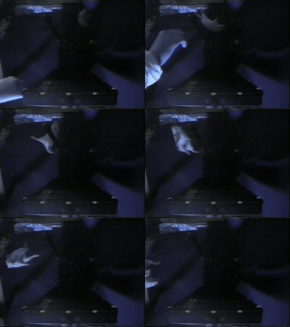
Source: NASA Neurolab mission footage
Their findings, published in Nature Neuroscience, showed that hippocampal neurons can form robust, spatially selective firing fields even in the absence of gravitational cues, but that the process may require more time or experience than under normal terrestrial conditions.
The Experiment
The rats were implanted with chronic multi-electrode recording arrays targeting hippocampal area CA1. On the shuttle, they navigated two track configurations:
- The Escher Staircase, a three-dimensional track with interleaved 90-degree yaw and pitch turns. A rat making three right turns would complete a full circuit and return to its starting position, something that would require four turns on a flat surface. This design put landmark-based spatial information in direct conflict with the internal sense of direction.
- The Magic Carpet, a flat, two-dimensional surface for comparison.
The rats pulled themselves along the tracks by grasping the edges, receiving medial forebrain bundle stimulation as a reward. Position was tracked via video camera, and spike data was sorted offline using Xclust.
Key Findings
Despite the absence of gravity, which renders the otolith organs useless for sensing static head orientation, place cells developed normal spatial firing properties:
- Spatial information content (bits per spike) on Flight Day 9 was statistically indistinguishable from preflight recordings for all three rats.
- Place fields were stable across repeated sessions on the same track.
- Some cells showed direction selectivity, firing preferentially when the rat moved in one direction, a property also seen on Earth.
- Hippocampal EEG showed normal theta rhythm during locomotion and normal sharp waves and ripples during rest.
Interestingly, the first exposure to the Escher Staircase on Flight Day 4 produced abnormal spatial firing patterns that differed between rats, suggesting that the hippocampus may need either a period of adaptation to microgravity or more experience with a novel environment than is typically required on Earth.
Now Available on DANDI
Over 25 years after these historic recordings, the data is now publicly available on DANDI as Dandiset #001754. The NWB dataset includes:
- 8 NWB files across 3 rats, covering preflight and in-flight sessions (Flight Days 4 and 9)
- Spike-sorted unit data from multi-tetrode recordings in hippocampal CA1
- Position tracking for in-flight behavioral sessions
- Pre-computed rate maps (64x64 spatial firing rate maps) from the original analysis
- Behavioral epochs annotated with task type (Escher Staircase, Magic Carpet, Baseline)
All data is stored in the Neurodata Without Borders (NWB) format and can be streamed directly from DANDI, no download required. The original source data is archived on the NASA Open Science Data Repository (OSD-968), where it was curated by Rachel Gilbert, PhD, and Ryan T. Scott, PhD, of the NASA data curation team.
Explore the Data Yourself
We’ve prepared a Jupyter notebook that walks through the dataset and reproduces key analyses from the paper. Using pynapple for neural data analysis and remfile for streaming access, the notebook demonstrates how to:
- Stream NWB files directly from DANDI
- Visualize animal trajectories on the Escher Staircase, Magic Carpet, and Baseline tracks
- Plot spike rasters across all recorded neurons
- Compute 2D spatial firing rate maps and compare them against the pre-computed maps from the original analysis
- Compare place fields across different track geometries
The notebook confirms that place fields computed from the raw data closely match the pre-computed rate maps from over 25 years ago, a testament to both the quality of the original recordings and the value of standardized data formats for long-term preservation.
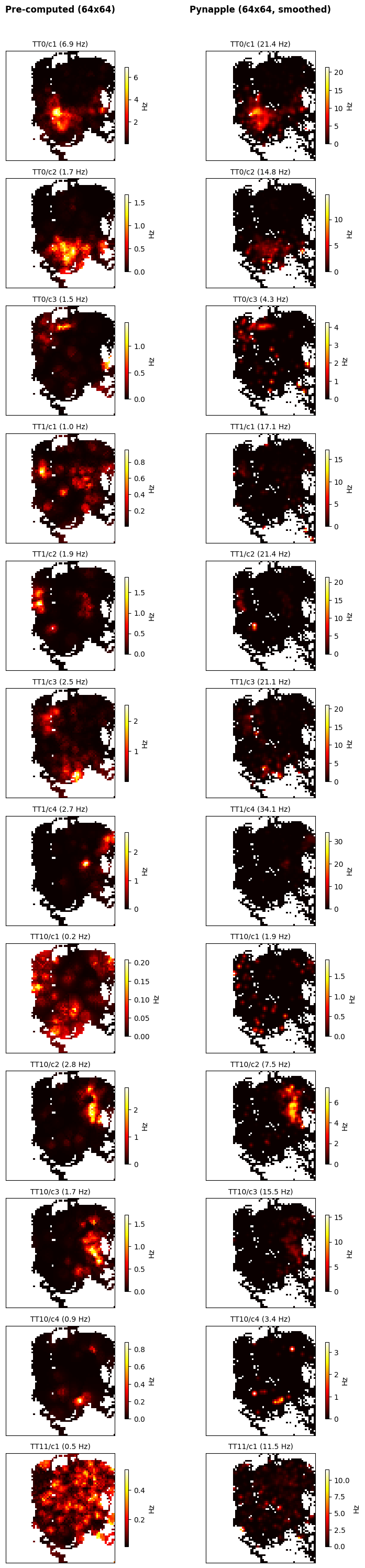
Reproducing spatial firing rate maps. Pre-computed rate maps from the original 1998 analysis (left) compared with rate maps computed from the raw spike and position data using pynapple (right). Each row is a single neuron recorded on the Escher Staircase track during Flight Day 9. Despite differences in peak firing rate due to smoothing parameters, the spatial structure of the place fields matches closely across both methods.
Why This Matters
This dataset is a unique piece of scientific history. While earlier COSMOS/Bion missions recorded vestibular neural activity from restrained monkeys in orbit, the Neurolab recordings remain, to our knowledge, the only cognitive neural data from freely behaving animals in space. The questions they raise are still open: Does the hippocampus develop a true three-dimensional spatial code in microgravity, or does it create independent two-dimensional maps for each surface? What cues drive place cell firing when gravity is absent? How does the vestibular system adapt during extended spaceflight?
By making this data openly available in a modern, standardized format, we hope to enable new analyses that were not possible with the tools of 1998. With renewed interest in long-duration spaceflight and the neuroscience of navigation, these recordings from the Space Shuttle may yet have more to teach us.
References
Knierim, J. J., McNaughton, B. L. & Poe, G. R. Three-dimensional spatial selectivity of hippocampal neurons during space flight. Nature Neuroscience 3, 209-210 (2000). doi:10.1038/72910
Introducing DANDI Atlas Explorer: Explore the DANDI Archive in 3D
Where in the brain does DANDI have data? As the archive grows, this question becomes increasingly important for researchers planning experiments, searching for collaborators, or surveying available data for meta-analyses. Today, we’re excited to introduce DANDI Atlas Explorer—an interactive 3D brain viewer that lets you explore the DANDI Archive through the lens of the Allen Common Coordinate Framework (CCF) mouse brain atlas.
What is DANDI Atlas Explorer?
DANDI Atlas Explorer is a browser-based tool that renders an interactive 3D mouse brain and highlights which regions have associated neurophysiology datasets on DANDI. Regions with more datasets appear more opaque, giving you an immediate, intuitive sense of data coverage across the brain. Click any region to see the specific dandisets that recorded there, with direct links back to the DANDI Archive.
The tool currently covers 48 dandisets spanning 353 brain structures, with data automatically updated nightly from the archive.
Key Features
Interactive 3D brain visualization. Rotate, zoom, and pan a fully rendered mouse brain with 445 anatomical meshes from the Allen Institute. Orientation buttons let you snap to standard views—dorsal, ventral, anterior, posterior, left, and right.
Hierarchical brain region browser. A searchable, collapsible tree mirrors the Allen CCF structure hierarchy. Each region displays a badge with the number of associated dandisets, making it easy to identify regions with available data.
Region-to-dataset linking. Click any brain region to see all dandisets that recorded from that area. Each dandiset entry shows its title, subject count, and a direct link to the DANDI Archive. You can drill down further to see individual subjects and their recording locations.
3D electrode visualization. For electrophysiology datasets, DANDI Atlas Explorer extracts electrode coordinates from NWB files and renders them as 3D point clouds within the brain. Select a subject to see exactly where electrodes were placed, overlaid on the anatomical context.
Shareable URLs. The app encodes your current selection in the URL, so you can share a link that takes a colleague directly to a specific brain region or dandiset view.
How It Works
DANDI Atlas Explorer bridges two major neuroscience resources. Brain anatomy comes from the Allen Brain Atlas API, which provides the hierarchical structure graph and 3D mesh geometry for every brain region. Dataset metadata comes from the DANDI Archive, where NWB files store brain region annotations and electrode coordinates alongside the neurophysiology data.
A Python pipeline processes this data:
- It queries the DANDI API for all mouse (Mus musculus) dandisets.
- For each dandiset, it streams NWB files to extract brain region labels and electrode coordinates—without downloading the full files.
- It matches extracted region names to Allen CCF structure IDs.
- It aggregates statistics and generates static JSON files that power the frontend.
The frontend is built with Three.js for 3D rendering, with no framework dependencies. A GitHub Actions workflow runs the data pipeline nightly, so the atlas stays current as new datasets are published to DANDI.
Use Cases
- Planning experiments: Check what data already exists for your brain region of interest before starting a new study.
- Finding collaborators: Discover which labs have published data from the same brain areas you study.
- Meta-analysis: Quickly survey data availability across brain regions for cross-dataset analyses.
- Teaching: Use the interactive 3D brain to teach neuroanatomy in the context of real datasets.
- Data discovery: Browse the DANDI Archive spatially rather than by keyword search.
Try It Now
DANDI Atlas Explorer is open source and runs entirely in your browser—no installation required.
The source code is available on GitHub. Contributions, bug reports, and feature requests are welcome.
DANDI Atlas Explorer was developed by CatalystNeuro with support from the DANDI project.
NWB Compression Recommendations for DANDI Archive
When submitting large datasets to the DANDI Archive, it’s crucial to consider data compression options that can substantially reduce file sizes. Smaller files reduce the storage burden on the DANDI Archive and make datasets more convenient to download for users. Neurodata Without Borders (NWB) now supports two file format backends: HDF5 and Zarr. Both formats have built-in capabilities for chunking and compression that can break large datasets into smaller pieces and apply lossless compression to each chunk. This approach reduces file size without altering the dataset values.
DANDI recommends compressing large datasets, but the variety of algorithms and settings available can be overwhelming for NWB users unfamiliar with data engineering. This post aims to answer several common questions:
- By how much can the volume of my data be reduced?
- What compression options are available and how can I access them?
- Which compression algorithms and settings are optimal for my use case?
The answers depend on specific use cases, but our analysis provides general guidelines to help you make informed decisions based on three key metrics: file size, read speed, and write speed. You may also need to consider accessibility - whether the HDF5 or Zarr library can read your file out of the box or requires installation of a dynamic filter.
When considering a compression algorithm, you should consider the following trade-offs:
- File Size: Higher compression levels typically yield smaller files but may require more time to compress and decompress.
- Read Speed: Some algorithms prioritize fast decompression, which is beneficial for users frequently accessing the data.
- Write Speed: If you frequently write or update data, faster compression algorithms may be preferable, even if they result in larger file sizes.
- Accessibility: Some compression algorithms are built into HDF5 and Zarr libraries, while others require additional installations. Choosing widely supported algorithms can enhance data accessibility.
Our Testing Approach
We conducted an evaluation of several popular compression algorithms in HDF5 using the h5plugin library, which simplifies the installation process for various compression algorithms and makes them available to h5py. For Python users, we highly recommend this package.
For our test data, we used action potential recordings from a Neuropixel probe (SpikeGLX acquisition system) from DANDI:000053, consisting of high-pass voltage data prior to spike-sorting. This represents a common use case for NWB files. While this analysis focuses on HDF5, similar compression principles apply to Zarr backends as well. We relied on h5py to automatically determine chunk shapes, with shuffle turned off.
Understanding Compression Algorithms
Before diving into the results, it’s helpful to understand the different compression algorithms tested and how they relate to each other:
Core Algorithms
gzip: A widely-used compression algorithm based on the DEFLATE method. It’s built directly into HDF5, making it the most accessible option (no additional libraries needed). Gzip prioritizes compression ratio over speed and has been a standard for decades.
zstd (Zstandard): A modern compression algorithm developed by Facebook that offers an excellent balance between compression ratio and speed. It provides adjustable compression levels (higher levels = better compression but slower) and has become increasingly popular for scientific data.
lz4: Designed primarily for speed, LZ4 prioritizes extremely fast compression and decompression at the cost of somewhat lower compression ratios. It’s ideal when read/write performance is the primary concern.
Blosc Meta-Compressor
Blosc is not a compression algorithm itself, but rather a meta-compressor that adds additional optimizations on top of existing compression algorithms. Blosc splits data into smaller blocks and applies multi-threading, which can significantly improve performance for large arrays. When you see “blosc” in our results:
- blosc zstd: Blosc wrapper around the Zstandard algorithm
- blosc lz4: Blosc wrapper around the LZ4 algorithm
- blosc zlib: Blosc wrapper around the zlib algorithm (similar to gzip)
- blosc blosclz: Blosc’s own compression codec
- blosc lz4hc: Blosc wrapper around LZ4 in “high compression” mode
The blosc-wrapped versions often show different performance characteristics than their standalone counterparts due to Blosc’s blocking and multi-threading optimizations, which can be particularly effective for numerical arrays like neurophysiology data.
Additional Resources
For those interested in learning more about compression principles and their application to scientific data:
- Data Compression Explained - Comprehensive introduction to data compression fundamentals
- Blosc Documentation - In-depth explanation of the Blosc meta-compressor
- HDF5 Filters - Technical details on how HDF5 implements compression filters
Results and Recommendations
 Figure 1: Comparison of compression algorithms. The black circle shows data that is chunked but not compressed. Each color represents a different algorithm, with lightness/darkness indicating compression level.
Key Findings:
Best Overall Performance: zstd level 3
- Provides excellent compression ratio (about 45% reduction)
- Maintains good read and write speeds at moderate compression levels
- At higher levels, write time increases dramatically with minimal additional space savings
Fastest Read Performance: blosc lz4
- If optimizing primarily for read speed, blosc lz4 is about twice as fast as zstd
- For blosc lz4, level 3 or 5 offers a good balance between size and speed
Alternative Option: gzip
- Most accessible because it is built into HDF5 (no additional configuration needed)
- Read time is about 1.8x slower than zstd
- At moderate levels (e.g., the default level 4), offers similar file size and write time to zstd
- Good option for users unable to configure custom dynamic filters
Best Compression Ratio: blosc zstd
- Achieves slightly better compression ratio and slightly worse read time than standard zstd
- Significantly longer write times at higher compression levels
Detailed Results
For those interested in the exact benchmark numbers, the table below shows all tested compression configurations with their corresponding write times, file sizes, and read times:
| name | write time (s) | file size (MB) | read time (s) |
|---|---|---|---|
| no_filter None | 0.170 | 768.009 | 0.098 |
| zstd (0,) | 1.857 | 387.450 | 1.005 |
| zstd (3,) | 3.222 | 354.957 | 1.289 |
| zstd (6,) | 8.464 | 347.277 | 1.339 |
| zstd (9,) | 14.810 | 345.556 | 1.278 |
| lz4 (0,) | 1.605 | 572.530 | 1.021 |
| lz4 (1000.0,) | 1.425 | 696.795 | 0.916 |
| lz4 (1000000.0,) | 1.589 | 572.530 | 1.107 |
| gzip 1 | 4.688 | 359.142 | 2.072 |
| gzip 4 | 8.018 | 346.226 | 2.099 |
| gzip 9 | 60.077 | 352.872 | 2.184 |
| lzf None | 1.607 | 527.347 | 0.982 |
| blosc blosclz 1 | 0.650 | 768.438 | 0.341 |
| blosc blosclz 3 | 1.183 | 684.614 | 0.653 |
| blosc blosclz 5 | 1.175 | 684.614 | 0.604 |
| blosc blosclz 7 | 1.846 | 617.389 | 0.819 |
| blosc blosclz 9 | 2.432 | 574.626 | 1.004 |
| blosc lz4 1 | 1.442 | 650.519 | 0.553 |
| blosc lz4 3 | 1.635 | 614.405 | 0.591 |
| blosc lz4 5 | 1.721 | 598.747 | 0.589 |
| blosc lz4 7 | 1.839 | 581.546 | 0.619 |
| blosc lz4 9 | 1.959 | 567.020 | 0.621 |
| blosc lz4hc 1 | 3.612 | 536.971 | 0.576 |
| blosc lz4hc 3 | 7.567 | 487.303 | 0.565 |
| blosc lz4hc 5 | 11.790 | 470.780 | 0.533 |
| blosc lz4hc 7 | 13.138 | 469.490 | 0.560 |
| blosc lz4hc 9 | 13.091 | 469.482 | 0.552 |
| blosc zlib 1 | 5.289 | 371.400 | 2.118 |
| blosc zlib 3 | 7.699 | 356.136 | 2.012 |
| blosc zlib 5 | 21.409 | 364.851 | 2.321 |
| blosc zlib 7 | 45.256 | 361.311 | 2.158 |
| blosc zlib 9 | 50.259 | 360.995 | 2.147 |
| blosc zstd 1 | 1.839 | 394.557 | 0.960 |
| blosc zstd 3 | 5.508 | 344.206 | 1.355 |
| blosc zstd 5 | 14.713 | 345.752 | 1.215 |
| blosc zstd 7 | 45.198 | 333.719 | 1.328 |
| blosc zstd 9 | 108.811 | 324.897 | 1.509 |
Conclusion
By applying appropriate compression settings to your NWB files before uploading to DANDI, you can significantly reduce storage requirements and improve download experiences for users of your datasets. For most neurophysiology datasets using the HDF5 backend, we recommend zstd level 3 or 4 as a good default that balances compression ratio with performance. However, if you have specific requirements for read speed or file size, you might consider blosc lz4 or blosc zstd respectively.
While this analysis focused on HDF5, Zarr offers similar compression options and benefits. Zarr natively supports blosc, zstd, and gzip compression algorithms with comparable performance characteristics. This is an active area of research, and there are newer algorithms that are designed specifically for electrophysiology and available in Zarr. See Compression strategies for large-scale electrophysiology data for a detailed discussion of these algorithms.
Remember that optimal compression settings may vary depending on your specific data characteristics and usage patterns. We encourage you to experiment with different options using the provided code example to find the best configuration for your datasets.
Code
import os
import hdf5plugin
import h5py
import time
from tqdm import tqdm
import matplotlib.pyplot as plt
from matplotlib.lines import Line2D
import json
import pandas as pd
import seaborn as sns


# set up parameters for tests
filters = {
    'no_filter': dict(
        filter_class={'chunks':(10000, 384)},
        compression_opts_list=[None],
    ),
    'zstd': dict(
        filter_class=hdf5plugin.Zstd(),
        compression_opts_list=[
            (0,),
            (3,),
            (6,),
            (9,),

        ],
    ),
    'lz4': dict(
        filter_class=hdf5plugin.LZ4(),
        compression_opts_list=[
            (0,),
            (1e3,),
            (1e6,),
        ],
    ),
    'gzip': dict(
        filter_class=dict(compression='gzip'),
        compression_opts_list=[
            1, 4, 9
        ]
    ),
    'lzf': dict(
        filter_class=dict(compression='lzf'),
        compression_opts_list=[None,],
    )
}


blosc_filters = ["blosclz", "lz4", "lz4hc", "zlib", "zstd"]

results = []


def test_filter(run_name, **kwargs):
    """Get write time, read time, and file size for a run."""

    fname = f"{run_name}.h5"


    with h5py.File(fname, mode="w") as file:
        start = time.time()
        file.create_dataset(**kwargs)
        write_time = time.time() - start

    file_size = os.stat(fname).st_size / 1e6

    with h5py.File(fname, mode="r") as file:
        start = time.time()
        data = file['data'][:]
        read_time = time.time() - start

    return {
        'name': run_name,
        'write time (s)': write_time,
        'file size (MB)': file_size,
        'read time (s)': read_time,
    }

def create_mini_palette(color, filter_, compression_opts_list):
    """Create palette of different shades of the same color for a given filter."""

    mini_pallete = sns.light_palette(
    color=color,
    n_colors=len(compression_opts_list)+2)[2:]
    for comp_opts, this_color in zip(compression_opts_list, mini_pallete):
        palette.update({f"{filter_} {comp_opts}": this_color})
    return palette


import lindi

# Load https://api.dandiarchive.org/api/assets/ac23d031-019a-4c07-854d-20a3647f3097/download/
local_cache = lindi.LocalCache()

file = lindi.LindiH5pyFile.from_lindi_file("https://lindi.neurosift.org/dandi/dandisets/000053/assets/ac23d031-019a-4c07-854d-20a3647f3097/nwb.lindi.json", local_cache=local_cache)

data = file['acquisition/ElectricalSeries/data'][:1000000]
print(f"{data.nbytes / 1e9} GB", flush=True)


## run filters

#test non-blosc filters
for filter_name, filter_dict in tqdm(list(filters.items()), desc='non-blosc'):
    args = dict(
        name="data",
        data=data,
        **filter_dict["filter_class"]
    )
    for compression_opts in filter_dict["compression_opts_list"]:
        args.update(compression_opts=compression_opts)
        run_name = f"{filter_name} {compression_opts}"
        results.append(test_filter(run_name, **args))

# test blosc filters
for filter_name in tqdm(blosc_filters, desc='blosc'):
    for level in range(1, 10, 2):
        args=dict(
            name="data",
            data=data,
            **hdf5plugin.Blosc(cname=filter_name, clevel=level, shuffle=0)
        )
        run_name = f"blosc {filter_name} {level}"
        try:
            results.append(test_filter(run_name, **args))
        except Exception as e:
            print(f"Error occurred for {run_name}: {e}")


df = pd.DataFrame(results)

# Calculate compression ratio (original size / compressed size)
original_size_mb = data.nbytes / 1e6
df['compression ratio'] = original_size_mb / df['file size (MB)']

df.to_parquet("results.parquet")

# uncomment for previous results
# df = pd.read_parquet("results.parquet")

# Save results as HTML table
df.to_html("results.html", index=False, float_format=lambda x: f'{x:.3f}')

# visualization - construct palette

# for non-blosc
counter = 0
base_palette = sns.color_palette(n_colors=11)
palette = {'no_filter None': 'k'}
for filter_, filter_dict in list(filters.items())[1:]:
    color = base_palette[counter]
    if filter_ not in ('no_filter None',):
        palette.update(create_mini_palette(color, filter_, filter_dict["compression_opts_list"]))
    counter += 1


# for blosc
for filter_name in blosc_filters:
    counter += 1
    color = base_palette[counter]
    palette.update(create_mini_palette(color, "blosc " + filter_name, range(1, 10, 2)))

n_filters = sum(len(x["compression_opts_list"]) for x in filters.values())
n_blosc_filters = 7*len(blosc_filters)
markers = ['o'] * n_filters + ['x'] * n_blosc_filters

# Create PairGrid without diagonals
g = sns.PairGrid(data=df, hue="name", palette=palette, corner=True, height=4, diag_sharey=False)

# Map scatter plots to lower triangle with custom markers
def scatter_with_markers(x, y, **kwargs):
    """Custom scatter function that uses different markers for blosc vs non-blosc."""
    data = kwargs.pop('data')
    hue = kwargs.pop('hue', None)

    for name in data[hue].unique():
        subset = data[data[hue] == name]
        marker = 'x' if name.startswith('blosc') else 'o'
        color = palette.get(name, 'gray')
        plt.scatter(subset[x.name], subset[y.name], marker=marker, c=[color],
                   s=30, alpha=0.6, label=name)

# Use custom function for lower triangle
for i in range(len(g.axes)):
    for j in range(len(g.axes[i])):
        if i > j:  # Lower triangle only - plot data
            ax = g.axes[i, j]
            x_var = g.x_vars[j]
            y_var = g.y_vars[i]

            for name in df['name'].unique():
                subset = df[df['name'] == name]
                marker = 'X' if name.startswith('blosc') else 'o'
                color = palette.get(name, 'gray')
                ax.scatter(subset[x_var], subset[y_var], marker=marker, c=[color],
                          s=30, alpha=0.6, label=name)

            ax.set_xlabel(x_var)
            ax.set_ylabel(y_var)
        elif i == j:  # Diagonal - remove these axes
            g.axes[i, j].remove()

# Add legend with custom markers
handles = []
labels = []
for name in df['name'].unique():
    marker = 'X' if name.startswith('blosc') else 'o'
    color = palette.get(name, 'gray')
    handles.append(Line2D([0], [0], marker=marker, color='w',
                         markerfacecolor=color, markersize=8, alpha=0.6))
    labels.append(name)

g.fig.legend(handles, labels, loc='center right', bbox_to_anchor=(0, 0.5), ncol=2)

plt.savefig("eval_compressions.pdf", bbox_inches="tight")
plt.savefig("eval_compressions.png", bbox_inches="tight", dpi=300)
Unraveling Anesthesia's Effect on Brain Activity
Data Reuse Highlight:
This blog entry is part of an ongoing series that showcases examples of data reuse and reanalysis using publicly available data on DANDI.The Original Study: Peering into the Anesthetized Brain
In June 2023, Dr. Leslie Claar and colleagues from the Allen Institute published their groundbreaking findings in the journal eLife in the article, “Cortico-thalamo-cortical interactions modulate electrically evoked EEG responses in mice”. Their approach was comprehensive: they stimulated mouse cortex while simultaneously recording with electroencephelography (EEG) and neuropixels probes, comparing brain activity during wakefulness and under isoflurane anesthesia.
In awake mice, Claar’s team observed a robust event-related potential (ERP) when they delivered pulsatile electrical stimulation to deep layers of the motor cortex (Figure 1A left). This ERP coincided with a distinct pattern of neural spiking, both locally in the motor cortex and in distant sensorimotor-related thalamic nuclei (Figure 1B left). The response followed a three-act play: initial excitation within 25 milliseconds, a period of quiescence for about 125 milliseconds, and finally, a strong rebound excitation before returning to baseline. When the mice were under anesthesia, the story changed dramatically. The ERP’s amplitude and complexity plummeted in response to the same stimulation (Figure 1A right). While the initial excitation persisted in the motor cortex, it vanished in the thalamic nuclei (Figure 1B right). The rebound excitation, along with its corresponding ERP component at around 180 milliseconds, was significantly weakened.
Based on these observations, Claar and colleagues proposed that interactions between the cortex and thalamus are responsible for the rebound excitation phase of the stimulus response. This rebound excitation, in turn, drives the second component of the ERP – a crucial signal of wakefulness.
After their experiments, Claar and her team published their data on DANDI, ensuring that it would remain publicly accessible for any future researchers who wanted to use it. The dataset and manuscript were prepared and published concurrently, which ensured that the dataset included all the paper-relevant data and metadata and curious reviewers could inspect the data directly if they so wished.

Figure 1: Brain state modulates the ERP via cortico-thalamo-cortical interactions. (A) Butterfly plot of ERPs during non-running (quiet wakefulness), running (active wakefulness), and isoflurane-anesthetized states. (B) Normalized firing rate, reported as a z-score of the average, pre-stimulus firing rate, of all RS neurons recorded by the Neuropixels probes targeting the stimulated cortex (MO) and SM-TH. Reproduced from “Cortico-thalamo-cortical interactions modulate electrically evoked EEG responses in mice”.
A New Perspective: Zooming in on Synaptic Potentials
Just a few months later, in November 2023, Drs. Richard Burman, Paul Brodersen and colleagues at the University of Oxford wrote a paper that included reanalysis of this data. Their findings were published in the journal Neuron with the article, “Active cortical networks promote shunting fast synaptic inhibition in vivo”. They also investigated the effects of anesthesia on brain activity, but narrowed their focus to the differential function of a specific receptor subtype: GABAAR.
Burman and Brodersen’s team used a technique called in vivo gramicidin perforated patch-clamp recording, combined with optogenetic activation of GABAergic synaptic inputs. They compared the GABAA receptor equilibrium potential (EGABAAR) in mice during wakefulness and under urethane anesthesia.
Their findings were striking. In anesthetized mice, GABAA receptor responses were significantly hyperpolarizing, with an average equilibrium potential of -80.8mV. In awake mice, however, these responses could be either hyperpolarizing or depolarizing, averaging at -63.9mV – a state known as the “shunting” regime.
Burman et al. hypothesized that the higher network activity in the awake state leads to a higher concentration of intracellular chloride, which in turn depolarizes the GABAA receptor equilibrium potential. Anesthesia, by broadly suppressing neural activity, indirectly hyperpolarizes EGABAAR. They confirmed this hypothesis by locally injecting an AMPA receptor antagonist (NBQX) which suppressed network activity, and hyperpolarized EGABAAR to -78.0mV.
The Oxford researchers also hypothesized that changes in EGABAAR would lead to changes in network activity, resulting in a bi-directional relationship between the two quantities.
To test this hypothesis, Burman and Brodersen’s team turned to the data from Dandiset #000458 – the very same dataset used by Claar et al. By reanalyzing this data and manipulating a computational network model, they found that setting the EGABAAR parameter to the shunting regime (-60mV) reproduced spiking responses similar to those seen in awake mice (Figure 2 B&F left). Conversely, setting it to the hyperpolarizing regime (-80mV) mimicked the responses seen in anesthetized mice (Figure 2 B&F right). This data provides evidence for the hypothesized bidirectional relationship.

Figure 2: Shunting inhibition promotes local network desynchronization and response flexibility. (A) High-density Neuropixels (NPXs) recordings were used to compare spiking activity in the same cortical neurons under awake and anesthetized conditions. (B) Example raster plots show the spiking activity of a population of neurons in somatosensory cortex (SS). Spiking activity is shown across three stimulation trials for each condition. (C) Neuronal synchrony on a trial-to-trial basis (top) and the entropy of the peri-stimulus histogram (bottom) were calculated for each of the 662 recorded neurons under awake and anesthetized conditions (17 probe recordings in 16 mice). Each dot corresponds to a single neuron and the dashed line indicates the line of equality. (D) Neurons in the awake condition exhibited lower synchrony (top; Aw.: 0.325 ± 0.005 vs. An.: 0.393 ± 0.007, p < 0.001, paired t test) and higher entropy (bottom; Aw.: 1.347 ± 0.018 nats vs. An.: 1.111 ± 0.020 nats, p < 0.001, paired t test). (E) Schematic of network model consisting of interconnected excitatory pyramidal neurons (Pyr.) and inhibitory interneurons (IN). EGABAAR in the pyramidal neurons was adjusted relative to the RMP to create two different conditions: a shunting (Shunt.) and a hyperpolarizing (Hyperpol.) EGABAAR condition. Spiking activity was evoked by delivering brief depolarizing currents (input) of varying amplitudes to each neuron in the network. (F) Raster plots for the same population of pyramidal neurons (n = 50) in the shunting (left) and hyperpolarizing (right) EGABAAR conditions. (G) Synchrony (top) and entropy (bottom) for pyramidal neurons in the shunting and hyperpolarizing EGABAAR conditions (n = 1,000 randomly selected). Dashed line indicates the line of equality. (H) Neurons in the shunting EGABAAR condition exhibited lower synchrony (Shunt: 0.784 ± 0.001 vs. Hyperpol: 0.881 ± 0.001, p < 0.001, paired t test) and higher entropy (Shunt: 0.451 ± 0.002 nats vs. Hyperpol: 0.197 ± 0.002 nats, p < 0.001, paired t test) (n = 16,000 pyramidal neurons from the model). ∗∗∗p < 0.001. MO, motor cortex; Stim., electrical stimulation; TH, thalamus. Reproduced from “Active cortical networks promote shunting fast synaptic inhibition in vivo”.
Bridging Scales: From Synapses to Networks
Together, these two studies provide a rich, multi-level account of what happens to brain activity under anesthesia. They span from macroscale brain signals recorded by EEG all the way down to microscale synaptic responses from a single receptor type. The population spiking data from Dandiset #000458 serves as a crucial bridge between these levels, allowing Burman et al. to explicitly connect their work to the broader field of anesthesia research.
However, it’s important to note some key differences between the two studies. Claar et al. used isoflurane anesthesia and stimulated layers 5/6 of the cortex, while Burman et al. used urethane anesthesia and recorded from layer 2/3. Additionally, while Claar et al. found the most dramatic differences between waking and anesthetized states around 180 ms after stimulation, Burman et al. focused their reanalysis on the initial spiking response within 15 ms of stimulation.
These differences highlight the potential for further reanalysis of Dandiset #000458. Future studies could explore more similar experimental conditions, conduct a more thorough treatment of relevant response time periods, or investigate different aspects of anesthesia’s effects altogether.
Engaging with the Open Science Community
For those inspired by the work of Claar, Burman and Brodersen, and their teams, the journey doesn’t end here. We encourage readers from all backgrounds to take advantage of this open science platform by publishing and reanalyzing data on DANDI. We are confident that it will be a smooth and rewarding experience, but don’t just take our word for it – listen to what Dr. Leslie Claar and Dr. Paul Brodersen have to say,
“After organizing our dataset into NWB format, validating and uploading our files was straightforward using a few simple commands from the DANDI Python Client. The tools are well-documented, which made the process of uploading and publishing quite smooth. Within a few months of publishing on DANDI, others were already interested in using our dataset.” – Dr. Leslie Claar
“The DANDI archive is a fantastic resource with great tooling and exhaustive documentation. Its command line interface makes data retrieval and synchronization as simple as possible (but not simpler!). The standardized and well-documented formats for electrophysiological and neuroimaging data ensure that anyone can quickly find their way around a new archive without requiring extensive feedback from the authors that originally collected the data. These features make the DANDI archive a treasure trove of useful and reusable data, unlike the unfortunately still commonplace unstructured data dumps on many other platforms or – worst of all – university servers.” – Dr. Paul Brodersen and Professor Colin Akerman
To get you started on your own reanalysis project, we’ve prepared a Jupyter notebook demonstrating some basic reanalysis of Dandiset #000458. This tool will help you dive right into the data, guiding you through the initial steps of exploration and analysis. We have also prepared a Neurosift walkthrough which demonstrates how to use Neurosift to quickly and easily explore the NWB files in this dataset without even leaving the browser.
By engaging with this open science platform, you become part of a larger community of researchers who are building on each other’s work and driving the field forward. In the world of open science, collaboration and curiosity drive discovery—so why not see where the data takes you?
Human ex-vivo microscopy workshop/hackathon
Date/Time: April 21 - 22, 2022. 9am - 6pm ET
Online: Link will be sent to registered participants.
If you are interested in participating please fill in this form to be sent announcements: Register here
Pre-meeting presentations
- The Dandisets
- The Standards
- The Tools
Agenda for the hackathon
The events will run 9 - 6 ET to accommodate multiple time zones. Participants are welcome to join at any time.
Day 1: April 21, 2022 (9 - 6 ET)
DANDI+Microscopy Starter Kit: We will generate a set Starter Kit that makes it easy for users to navigate these and other Dandisets, including easier visualization of individual files.
Dandiset Abstraction Layer:
- Create a set of scripts to make it easy to programmatically access these Dandisets
- Be able to view and compute on them.
Unconference session (11.30 - 12.30 ET)
Day 2: April 22, 2022 (9 - 6 ET)
Visualization/Annotation:
- Develop a visualization of a single slab or a set of related chunks
- Develop the steps to annotate using NeuroTrAle
Registration:
- Develop scripts to register lightsheet data to MRI at different scales
Unconference session (11.30 - 12.30 ET)
Please feel free to comment on this community doc.
External Links in NWB and DANDI
The need for external files
Neurophysiology experiments often include natural videos (such as behaving animals), which need to be stored with the neurophysiological recordings in order to ensure maximal reusability of the data. These videos are commonly stored with lossy compression (e.g. h264 in an .mp4 file), which allows them to achieve very high compression ratios. It is possible to read these videos frame-by-frame, and store them in HDF5, but since HDF5 is not able to access popular video codecs like h264, the volume of the video in the NWB file is much larger (even when using the available compression algorithms like GZIP). NWB has an option to avoid storing these altogether by linking to these external video files using a relative path to that file on disk. This relative path is stored in the ImageSeries neurodata_type storing it as an attribute of a string dtype. We also need to publish these video linked NWB files in an archive (e.g. in DANDI). For DANDI, which renames and reorganizes the the NWB files, this requires not only uploading the video file on the archive but also changing the path attribute of the ImageSeries to reflect the new file names.
To implement this, we have created a formal naming convention for these video files relative to the NWB files’ path. In addition, these video files are also placed in a specific folder structure relative to the new location of the NWB file during the dandi organize call.
Internally the steps are as follows:
- Organizing and renaming the video files with one of move/copy/symlink/hardlink in the new folder structure.
- Updating the value of the
external_fileattribute in the NWB files. - Uploading on DANDI.
Note: this solution is specifically for natural videos like those of behaving animals. There are other types of image sequences like image stacks from optical physiology, which do not use codecs like h264; these types of videos can be copied into an HDF5 file.
Example re-organization
Original folder organization
├── nwbfiles
│   ├── test1_0_0.nwb
│   └── test1_1_1.nwb
└── video_files
    ├── test1_0.avi
    ├── test1_1.avi
    ├── test2_0.avi
    └── test2_1.avi
With the path attribute as: image_series.external_files=["../video_files/test1_0.avi", "../video_files/test1_1.avi"]
After dandi organize
The renaming pattern is as follows /<nwbfile_name>/{ImageSeries UUID}_external_file_{number}.mp4.
This UUID is that assigned to the ImageSeries datatype when its created. Thus its possible to lookup a video file linked to an NWB file and vice versa.
└── dandi_organized
    ├── sub-mouse0
    │   ├── sub-mouse0_ses-sessionid0_image
    │   │   ├── 933f8cf6-9e4b-405f-8cad-cc031d1fafc9_external_file_0.avi
    │   │   └── 933f8cf6-9e4b-405f-8cad-cc031d1fafc9_external_file_1.avi
    │   └── sub-mouse0_ses-sessionid0_image.nwb
    └── sub-mouse1
        ├── sub-mouse1_ses-sessionid1_image
        │   ├── 03137112-9d42-46b6-9046-45bc9aa7eb5e_external_file_0.avi
        │   └── 03137112-9d42-46b6-9046-45bc9aa7eb5e_external_file_1.avi
        └── sub-mouse1_ses-sessionid1_image.nwb
With the renamed path attribute as
image_series.external_files=
["sub-mouse0_ses-sessionid0_image/933f8cf6-9e4b-405f-8cad-cc031d1fafc9_external_file_0.avi",
"sub-mouse0_ses-sessionid0_image/933f8cf6-9e4b-405f-8cad-cc031d1fafc9_external_file_1.avi"]
Code Walkthrough
- Register dataset on DANDI (sandbox)
cd dandi_organized
dandi download "https://sandbox.dandiarchive.org/#/dandiset/101391/draft"
- Organize
cd dandi_organized
dandi organize -f "copy" --update-external-file-paths --media-files-mode "copy" "/nwbfiles"
–modify-external-file-fields option is a flag.
If active, the organise operation modifies the external_file field of an ImageSeries that holds the local location of an associated video file. It changes the value to the new name as per the convention above.
If no external_file field found in all nwb files, but this option is active, then it logs a warning.
If any NWB file’s ImageSeries has a external_file, but this option is not specified, then it raises a ValueError to avoid breaking the link.
–media-files-mode can be any of copy/move/symlink/hardlink.
This can only be specified if the –modify-external-file-fields flag is True. This is an optional argument, if not specified it defaults to “symlink”: an efficient way to deal with possibly large video files.
- Validate
dandi validate
- Upload
dandi upload -i dandi-sandbox "/dandi_organized"
Example dandiset here
- download
This dataset can then be downloaded using:
mkdir dandi_download
cd dandi_download
dandi download "https://sandbox.dandiarchive.org/#/dandiset/101391/draft"
The folder will contain all the video files along with the dandi metadata .yml and .nwb files.
DANDI User Workshop
Click to view a recording of the workshop
Registration is closed

DANDI: A data archive and collaboration space for neurophysiology
DANDI is a US BRAIN Initiative supported data archive for publishing and sharing neurophysiology data including intracellular and extracellular electrophysiology, optophysiology, and behavioral time-series, and images from immunostaining experiments. For example, data from experimental techniques like patch clamps, silicon probes, and calcium imaging can be published on DANDI. So can data from lightsheet microscopy experiments when combined with associated MRI data.
DANDI allows scientists to publish “dandisets,” collections of data from neuroscience experiments that are often associated with specific papers or projects. DANDI is built to scale with the growing data engineering needs of the community and can easily receive and publish TBs of data for free supported by the AWS public dataset program. It also uses best practices in metadata curation using the DANDI schema and allows users to mint DOIs using Datacite for publishing dandisets.
For neurophysiology data, DANDI supports the Neurodata Without Borders (NWB) standard. The NWB standard ensures that data is shared with the necessary metadata for reanalysis, allows for analyses that aggregate data across dandisets, provides a common platform for building analysis and visualization tools for published data, and allows DANDI to easily extract metadata to provide powerful detailed search features. For MRI and related data, DANDI has been leveraging the BIDS standards and working with other groups to extend support to microscopy and electrophysiology.
With DANDI Hub, DANDI is more than just an archive, but in fact an entire cloud-based collaborative platform, available for free to all DANDI users! DANDI Hub is a JupyterHub with access to high performance multi-core compute nodes and high-bandwidth access to all data hosted on DANDI. DANDI Hub provides many different workflows to interact with your data, including Python, R, and Julia Jupyter notebooks, a terminal, and even a Linux desktop view, all deployed for free and on demand in the cloud. The hub can be used to share code that reproduces key figures from papers, or to interactively explore any dandiset.
You can navigate all data conveniently using the Web app, or for more control we have several software tools for interacting with DANDI. The DANDI Python library and command line interface allows for performant upload, download, and querying. The DANDI REST API can also be used to interface with web applications. Also, all dandisets are made available using Datalad, which provides convenient data access across different systems.
Upload your data today! See our user guide for details. If you have any questions, please use our help desk and we will be happy to assist.